Advanced Simulator of Airborne Pathogen Propagation

Version: 1.5

Summary

ASAPP stands for Advanced Simulator of Airborne Pathogen Propagation. The ASAPP software developed by Buildwind combines high-quality computational fluid dynamics (CFD) simulation with advanced data processing to predict the probability of airborne infection.

This document addresses the fundamental concepts and models behind ASAPP and its use for airborne infection prediction and mitigation.

Introduction

The approach used by ASAPP consists of four main steps: the generation of a three-dimensional model , the definition of the problem conditions , the numerical solution of the governing equations, and the data analysis .

The three-dimensional CAD model includes all relevant room features: floor, walls, ceiling, doors, windows, and HVAC system. Elements such as furniture, technical equipment, and space occupants are also introduced.

Specialized numerical methods then transform this three-dimensional representation into a computational mesh, where the CFD code solves the governing equations describing the Physics of air motion, droplet motion, heat and mass transfer. Appropriate models are used in the ASAPP software to describe air turbulence, air properties (density, viscosity, and thermal conductivity), droplet drag, evaporation, and pathogen infectivity decay.

The solution of the case is done by employing an optimized CFD code developed by Buildwind, based on the standard OpenFOAM software. As a result of the high-quality three-dimensional model and the detailed physical description, the CFD simulations must be carried out on a high-performance computing system.

The obtained data are spatially filtered applying the ISO 18158:2016 definition of breathing zone. The time-dependent probability of infection is numerically integrated considering infectivity data from medical and biological literature for the pathogen that is being considered. The information is finally presented as colored maps to facilitate the interpretation of the results by the end user.

Computational models for ASAPP simulation

Computational fluid dynamics (CFD) is a powerful tool for the prediction and analysis of disease transmission by respiratory droplets. It has been used in many scientific works, such as (Borro et al. 2021), where the authors employ a multiphase approach to optimize the use of Local Exhaust Ventilation systems (LEV), hence decreasing the possibility of contagion of a hospitalized patient next to a spreader individual. CFD results are compared against the traditional Wells-Riley approach for airborne-driven transmission in (Foster and Kinzel 2021) . The results show that for an airborne pathogen, mask mandates, number of occupants, and proper HVAC operation drive protection from airborne pathogens, while physical distancing, on the other hand, has only a minor effect of reducing transmission.

ASAPP implements an unsteady particle tracking method to describe the droplets as lagrangian particles: air velocity, pressure, temperature and species are solved over all the numerical grid, while each droplet is introduced as an independent entity called a lagrangian particle

Fluid dynamics model

The time-evolving turbulent flow field is solved employing the URANS approach. The turbulence is modeled via SST model. The solution is obtained with a pressure-based solver and a PIMPLE algorithm. Second order schemes are used for the transported variables, and the Euler scheme is employed for time. In order to guarantee the correct particle displacement calculation, a pseudo time stepping for the lagrangian phase is employed. It takes as input the flow field time step and divides it on the basis of a limiting Courant-Friedrichs-Lewy Number and the particle's updated position. Buoyancy effects, e.g. around the bodies of the occupants, are taken into account.

Respiratory droplet model

The main input parameters for the droplet injection are the type of respiratory activity, i.e. breathing, coughing, sneezing or speaking, the temperature and composition of the droplets, and the duration and frequency of the events for each occupant. Once the droplets are introduced in space two most important phenomena take place, the variation in the droplet size due to mass exchange and the infectivity decay in time. In the following three aspects, namely the respiratory event particle distributions, the phase change modeling and the lifetime deactivation will be succinctly disclosed.

Droplet phase change

The criterion to apply evaporation modeling is based on (Nicas, Nazaroff, and Hubbard 2005). The equilibrium size corresponds to the diameter of a particle for which there is no net change in water content, that is, there is a balance between any evaporation of water vapor from and condensation to the particle. Due to the presence of solutes in an aqueous respiratory particle some water will remain in the particle at equilibrium unless the RH is very low (below the crystallization RH) and the equilibrium diameter will be larger than estimated for complete drying.

Instantaneous evaporation (no modeling)

Small sized particles quickly equilibrate to the surrounding environment being evaporation a rapid process (Holmgren et al. 2011). For particles with an initial diameter d 0 ≤ 20 µm, given the relatively short time scale (less than one second for RH between 30% and 70%), evaporation from respiratory particles is considered as an instantaneous process. Thus the particle distribution is assumed to correspond to the equilibrium diameter and no further evaporation is modeled.

Evaporation modeling

For particles with an initial diameter d 0 > 20 µm evaporation should be modeled. The equilibrium diameter for a particle of respiratory fluid containing glycoprotein over the typical range of indoor RH (30% to 70%), ranges from 0.47 × d 0 (30% RH) to 0.61 × d 0 (70% RH). The solid content is estimated such that the expression holds

d eq = 0.5×d 0 .

Conservation equations are written both for the droplet and the gas phase. In their interface the species and the heat flux are estimated via correlations, i.e. using the Sherwood and Nusselt numbers respectively. The mass and heat transfer modeling for forced convection, i.e. nonzero drop-gas velocity, is done in OpenFOAM via the Ranz-Marshall correlations:

Where , and are the droplet Reynolds, Schmidt and Prandtl numbers respectively.

The molar flux of vapor (kmol/m 2 /s) reads

where D v the vapor diffusivity, C s the vapor concentration on the droplet surface and that in surrounding gas. This takes into account the effect of the jet puff and of RH increase for dense sprays, which has proved to play an important role for particles with d 0 < 100 µm (Chong et al. 2021).

Respiratory events

Respiratory particle size distributions exhibit large within and between subject variability, as well as dependencies on respiratory activity, age and voice volume (Bagheri et al. 2023) . This holds for relatively steady events such as breathing as well as for violent expirations such as coughing and sneezing, which release multiphase turbulent flows that are generally composed of buoyant hot moist air and suspended droplets of various sizes (Bourouiba, Dehandschoewercker, and Bush 2014) . The ASAPP software contains a database with specific particle size distributions as a function of the chosen type of respiratory activity.

Breathing

The most recent particle size distribution proposed in (Bagheri et al. 2023) is employed, which covers droplets from 0.05 um up to 50 um. By means of a combination of particle size spectrometry and in-line holography the study offers a comprehensive data set covering the entire size range from nanometre to millimeter.

Figure 1 illustrates the particle size distribution used in ASAPP (Bagheri). A less recent distribution widely employed in scientific literature (Morawska et al. 2009) is shown as well, hence highlighting the improvement in droplet size resolution with the selected data set.

Figure 1: Comparison of two particle size distributions for breathing activity. Red curve (Bagheri et al. 2023) employed in the ASAPP software, blue line (Morawska et al. 2009).

The probability density function is numerically integrated to obtain the droplet concentration in terms of particle diameter. The outcome is subsequently discretized into a finite number of representative droplet bins, each one characterized by the corresponding mean Sauter diameter (d 32 ). A variable bin width is employed to guarantee the accuracy of the discretization, as the droplet concentration changes by a few orders of magnitude with increasing droplet diameter.

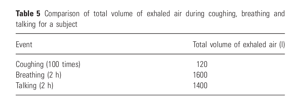
The breathing airflow rate from (Jitendra K. Gupta, Lin, and Chen 2010) is used within ASAPP.

Table 1: Comparison of total volume of exhaled air during coughing, breathing and talking for a subject (Jitendra K. Gupta, Lin, and Chen 2010) .

Speaking

The particle size distribution proposed in (Bagheri et al. 2023) for the condition speaking normal is used. For this respiratory activity the study detects particles in the range from 0.05 um up to 870 um. Figure 2 shows the substantial difference in the droplet concentration behavior for speaking with respect to breathing. The particle concentration at 10 um is one order of magnitude higher, and the largest droplets are also one order of magnitude larger. Moreover, there is a discrepancy among the speaking levels, i.e. normal and loud below 10 um, and this difference is reduced for the largest droplets.

Figure 2: Comparison of the particle size distributions for two different speaking levels and breathing (Bagheri et al. 2023).

The same methodology as for breathing is applied, namely, first the numerical integration to obtain the droplet concentration and subsequently the discretization into bins. The exhaled flow rate is estimated following the data in (Gupta et al. 2010).

Coughing

The distribution proposed in (Chao et al. 2009) is used. The authors suggest that the size distribution obtained at the 10 mm distance may essentially represent the ‘original' size distribution at the mouth opening, thus evaporation effects might be added subsequently.

Figure 3: Average droplet number count per person measured at the 10 and 60 mm distances (Chao et al. 2009) .

A time-varying profile is employed as in (J. K. Gupta, Lin, and Chen 2009) . The population is injected in the time range of 0.042–0.136 s, which represents only a fraction of the temporal velocity profile applied to the eulerian phase at the mouth of the spreader subject (Borro et al. 2021) .

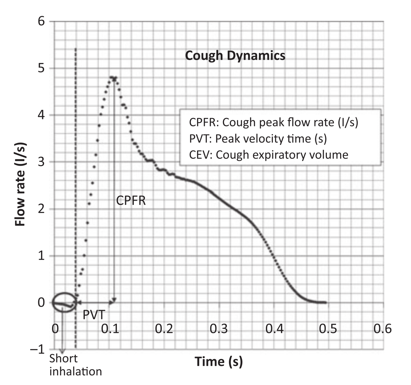
Figure 4: Cough ﬂow rate variation with time (J. K. Gupta, Lin, and Chen 2009) .

SARS-CoV2 infectivity decay

The infectivity decay is modeled as a function of the relative humidity. The range of exhaled breath relative humidity lies between 40-90% (Mansour et al. 2020) while the ambient values are a function of the considered space . The infectivity decreases to 10 % of the starting value after 20 min and a large proportion of the loss occurs within the first 5 minutes after aerosolisation . (Oswin et al. 2022) . A third degree polynomial function is used to regress the experimental data shown in the figure below from time zero up to 20 min. Subsequently the virus is considered to linearly diminish its infectivity and be able to remain viable in the air for up to 3 h post aerosolization (Buonanno, Stabile, and Morawska 2020) (Li et al. 2021) .

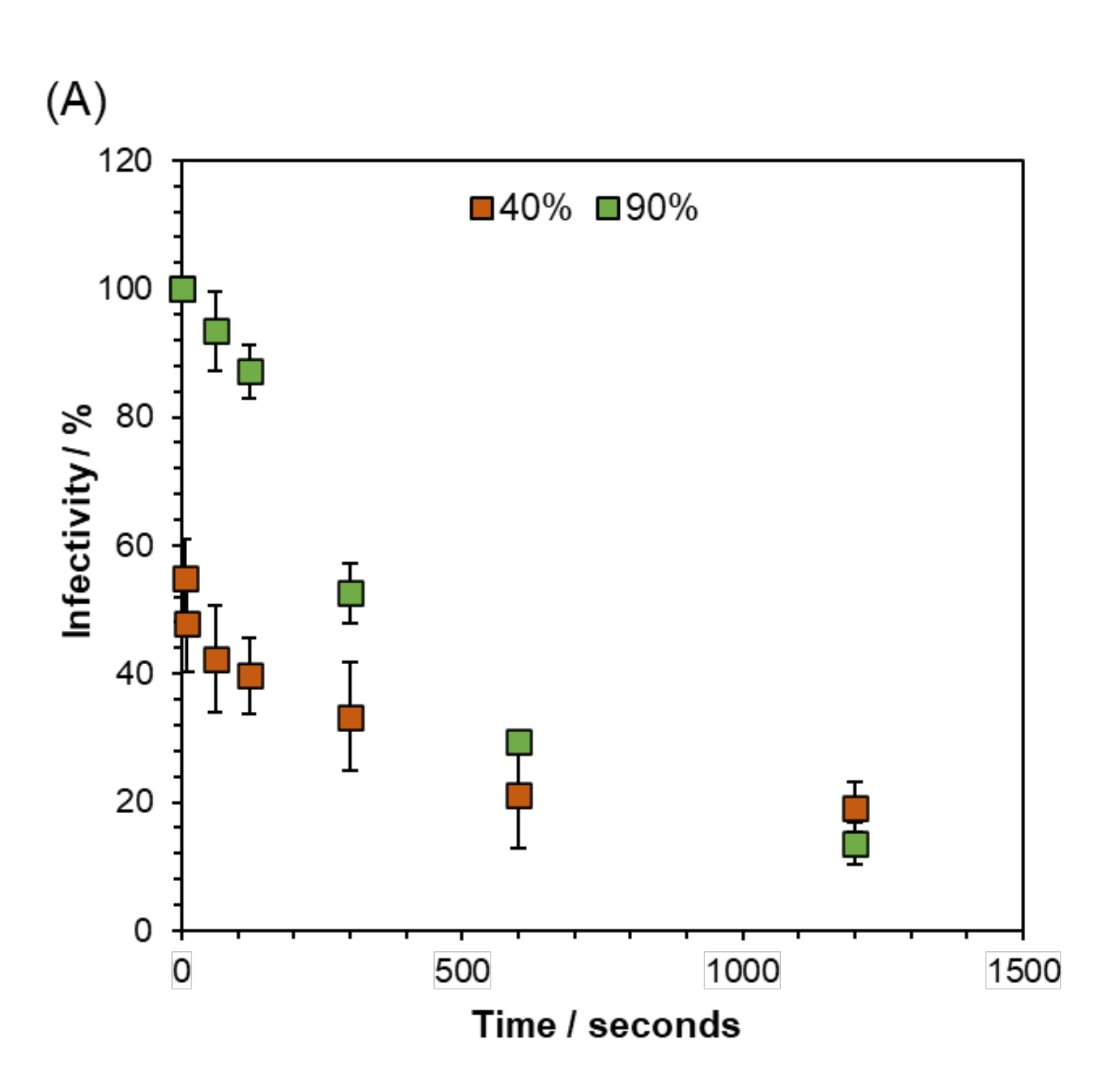
Figure 5: Short-Term Airborne Decay of SARS-CoV-2 from Oswin et al. 2022.

Computation of the probability of infection

ASAPP employs advanced algorithms to process the simulation results allowing for the detection of accumulation zones and the estimation of the probability of infection depending on the exposure and local concentration. The developed approach employs concepts from recent SARS-CoV2 studies, considering among others viral infectivity (Buonanno, Stabile, and Morawska 2020) , SARS-CoV2 multiphase modeling (Borro et al 2021), risk assessment based on CFD (Foster and Kinzel 2021) and risk assessment applied to SARS-CoV2 (Bazant and Bush 2021) , (Balachandar et al. 2020) , (Bourouiba 2021) .

The exhaled air concentration is modeled by means of a passive scalar. The boundary condition is set equal to one at the emission source, e.g. the person's mouth, and zero in the rest of the domain.

where corresponds to the Favre averaged exhaled air concentration , and is the effective diffusivity resulting from the molecular and turbulent components.

The aerosol concentration in the exhaled air reads

where is the droplet number concentration , the volume of a single droplet . For the current case two particle distributions have been used, breathing (Morawska et al. 2009) and coughing (Chao et al. 2009) .

The aerosol concentration in the flow field reads: (a widely used approach e.g. in Borro et al. 2021, Bazant and Bush 2021)

The average Lagrangian particle concentration within the breathing zone is the sum of the volume of all the droplets divided by the breathing zone volume

The ISO workplace air terminology defines the breathing zone as an hemisphere (generally accepted to be 30 cm in radius) extending in front of the human face, centered on the midpoint of a line joining the ears.The base of the hemisphere is a plane through this line, the top of the head and the larynx (ISO 18158:2016).

Figure 6: ISO standard breathing zones (Image source: OSHA.gov)

The average particle concentration within the breathing zone is the sum of the average lagrangian contribution plus the average aerosol concentration value within the region

The concentration of an infectious agent in the mouth (sputum) is assumed to coincide with that of the droplets emitted during the expiratory activities as in (Buonanno, Stabile, and Morawska 2020) .

A quantum is defined as the dose of airborne droplet nuclei required to cause infection in 63% of susceptible persons ( (Buonanno, Stabile, and Morawska 2020) ). The quanta density in a droplet reads

where is the viral load in the sputum , values have been proposed ranging between up to peak values of and a value of has been chosen to represent a realistic condition. a conversion factor defined as the ratio between one infectious quantum and the infectious dose expressed in viral RNA copies. Values have been suggested between and 0.1 was chosen for the case study following (Bazant and Bush 2021). This study highlights the relevance of the concentration of pathogens in the breath of an infected person and the relative transmissibility of the virus for risk assessment estimations. These values are expected to vary widely between different populations, among individuals during progression of the disease, and between different viral strains, so that further research is needed to improve the reliability of the predictions.

The mean quanta density , can be estimated as

Finally the inhaled quanta content from the flow field can be estimated as the product of the mean quanta density in the breathing zone and the inhaled volume

where the pulmonary ventilation rate for breathing is taken to be L/hr (Jitendra K. Gupta, Lin, and Chen 2010) .

The infectious probability is estimated considering the exhaled air and droplets quanta content, employing a Poisson distribution to make the result equivalent to the typical form of the Wells–Riley calculation as in (Foster and Kinzel 2021)

Validation of ASAPP software

Validation of ASAPP air flow and temperature prediction

The ability of the software to adequately describe the flow and temperature fields has been numerically validated against the experimental data presented in (Yin et al. 2009). The study analyzes displacement and mixing ventilation systems for a

patient ward, thus depicting relevant comparison scenarios for the ASAPP applications. Different ventilation conditions are achieved by changing both the air injection and the active exhaust devices. The experimental study employed rectangular boxes to represent the heat sources to eliminate errors that may be caused by complicated geometry. These heat sources include the patient (lying on the bed), the caretaker (standing next to him), medical equipment (behind the caretaker) and a television.

Figure 7: View of the patient ward CAD model.

The experiment utilized omnidirectional anemometers to measure the air velocity and temperature at eight poles around the patient bed and seven heights in each pole. The anemometers had an accuracy of 0.36°F for air temperature and 0.02 m/s for air velocity. Figures 7 and 8 compare the ASAPP software predictions for the temperature and velocity fields against the experimental data for the case of displacement ventilation with high level exhaust extraction for two different measurement poles.

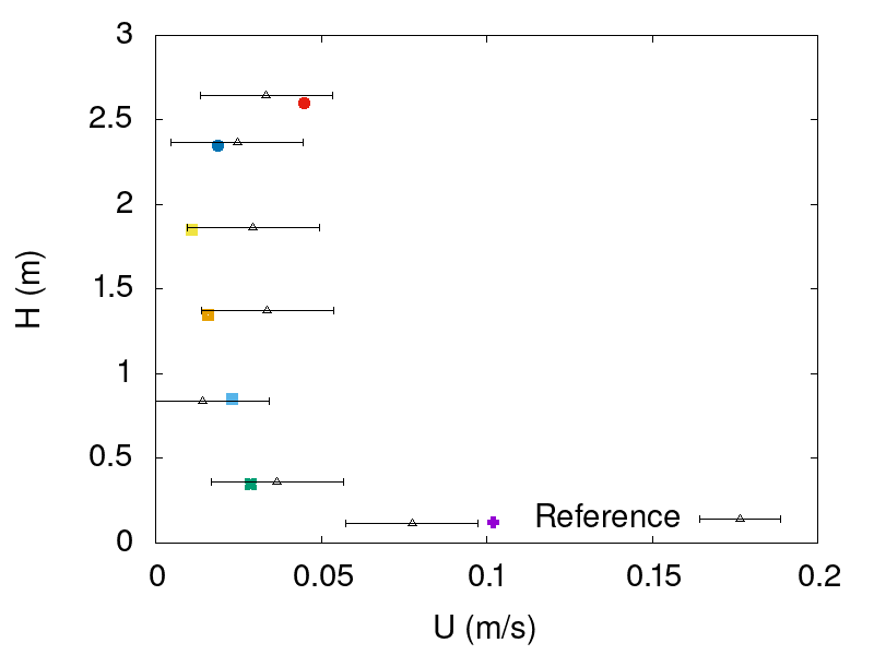
Figure 8: Comparison of ASAPP air velocity predictions (colored symbols) against the experimental data, at seven different heights for probes 1 and 5.

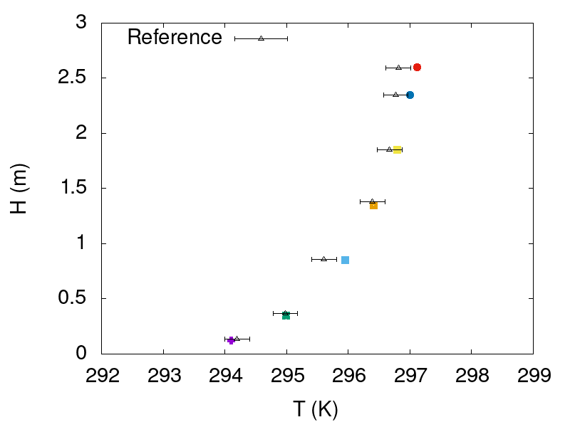
Figure 9: Comparison of ASAPP temperature predictions (colored symbols) against the experimental data, at seven different heights for probes 1 and 5.

Figures 8 and 9 show satisfactory agreement between ASAPP software predictions and experimental data. The deviations presented in the figures correspond to the measuring device uncertainty and not to deviations between different measurements. The results prove the ability of ASAPP software to adequately depict flow field behavior in indoor environments with heat transfer effects.

Validation of ASAPP infectivity prediction in hospital environment

CFD simulations using the ASAPP software were carried out to describe the droplet dynamics inside the CHU Liège hospital (Belgium) intensive care unit room for a SARS-CoV-2 patient. The simulations were carried out until the suspended droplet mass reached a steady condition. Subsequently, to assess the accuracy of the predictions samples were collected in locations having very high probability or very low probability of SARS-CoV-2 detection, as shown in figure 10.

Figure 10: prediction of droplet deposition on the floor and surfaces.

The cycle threshold or Ct value of a RT-PCR reaction is the number of cycles at which fluorescence of the PCR product is detectable over and above the background signal (Al Bayat et al. 2021) . A low Ct indicates a high concentration of viral genetic material, while higher Ct values indicate a low concentration of viral genetic material which is typically associated with a lower risk of infectivity ( Understanding Cycle Threshold (Ct) in SARS-CoV-2 RT-PCR: A Guide for Health Protection Teams 2020) . Detection of SARS-CoV-2 was done on 15 patients (naso-paryngeal PCR : Ct 9 to 33. For the current validation a Ct value lower than 20 was considered as positive, though standard RT-PCR might run up to 40 thermal cycles for virus detection (Rabaan et al. 2021).

For the patients found to be positive, two different techniques for environmental sampling were employed: the Sartorius portable air sampler for the droplets suspended in air and dry swabs for surface detection. The air sampler absorbs a defined volume of air through gelatin membrane filters that trap the virus, afterwards the culture-forming units per unit volume are calculated from the number of colonies growing on the culture medium in relation to the volume of air sampled. The experimental data was scrutinized using both univariate and multivariate analysis. Moreover the novel interactive and adaptive clinical decision support tool employing classification and regression tree analysis (CART) methodology proposed in (Saegerman et al. 2021) was applied for the data interpretation.

Figure 11 shows satisfactory agreement between the measurements and the ASAPP prediction . The left blue and orange columns indicate that the CFD adequately reckoned 11 out of 14 total positive measurements (both in air and on surfaces), while for the remaining three either it predicted no SARS-CoV-2 detection or a low concentration that could not be conclusive. In the opposite scenario, i.e. the determination of virus-free zones, (right orange and blue columns), the CFD results agreed with the experiments on 7 out of 8 samples, therefore delivering only one false positive. This demonstrates the capability of the ASAPP software to describe realistic conditions.

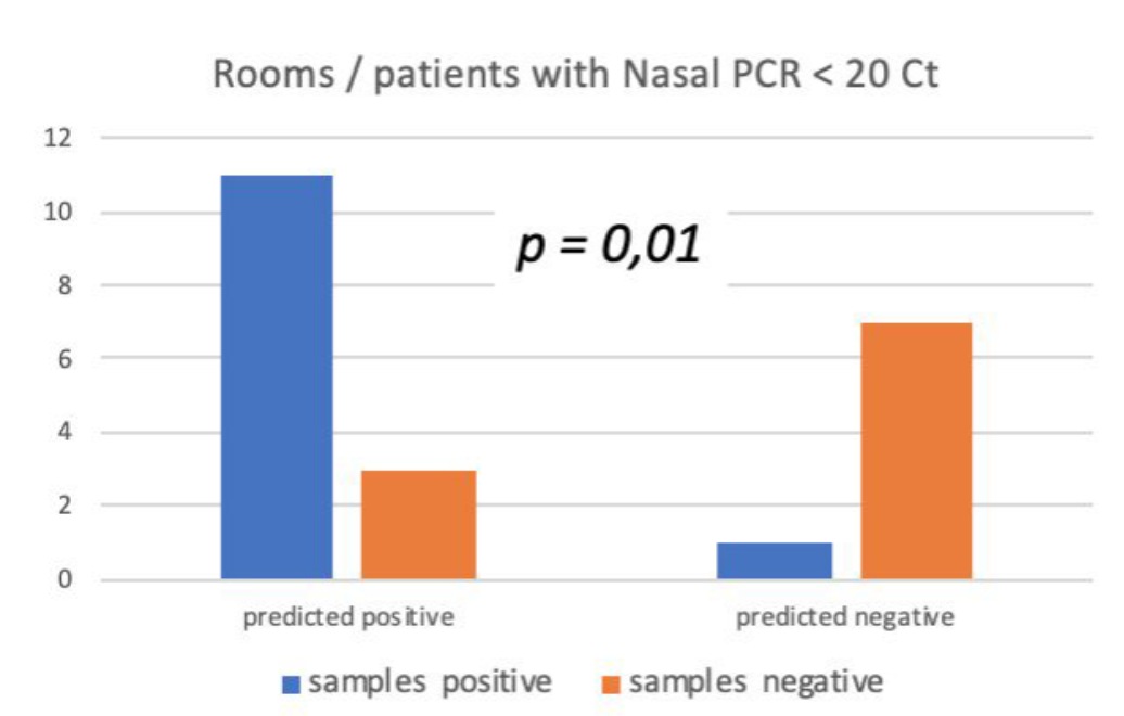
Figure 11: Agreement between the CFD predictions and the measurements.

Scientific contributions based on ASAPP software

Vega, P. J. O., Lucesoli, A., Mosca, G., Giulietti, R. A., D’Errico, M. M., & Gambale, A. (2024, April 24). Conversion of a regular patient room to negative pressure at Ancona university hospital (Italy). A combined experimental and numerical investigation. Building and Environment, 111557. https://doi.org/10.1016/j.buildenv.2024.111557.

Obando, P., Gambale, A., Mosca, G. RS Sampath Kumar. (2022, June 13-15). Application of computational fluid dynamics simulation to hospital room design to simultaneously predict air quality, airborne pathogen infection risk, and energy efficiency [Conference presentation]. European Healthcare Design 2022, London, England. European Healthcare Design.

De Harenne, C., Gambale, A., Obando, P., Bertrand, A., Misset, B. (2022, April 23-26). Prediction of the location of infectious droplets and aerosols in a patient intensive care room [Poster presentation]. European Congress of Clinical Microbiology and Infectious Diseases, Lisbon, Portugal. ECCMID 2022.

De Harenne, C., Obando, P., Kesseler, S., Pitti P., Lamtiri, M., Bertrand, A., Lisson, M., Haubruge, E., Gambale, A., Saegerman, C. Misset, B (2022, October 22-26). Prediction of the location of infectious particles in COVID-19 patient intensive care rooms, [Poster presentation]. 35th Annual Congress of the European Society of Intensive Care Medicine, Paris, France. 35th ESICM.

Misset B., De Harenne C., Kesseler S., Pitti P., Lamtiri M., Bertrand A., Lisson M., Haubruge E., Obando Vega P., Gambale A., Saegerman C. (2023, February 27-28). Prévention des infections aux soins intensifs : le COVID-19 dans un service réel. Journées de l’Architecture en santé, Brussels, 2023. JAS 2023.

D’Errico, M., Lucesoli, A., Allegrezza Giulietti, R., Bruschi, R., Martini, E., Salvi, A., Nitti, C., Talevi, G., Bertelli, F., Poniti, N., Gambale, A., Obando Vega, P., Mosca, G., Tavio, M., Airborne infection room retrofitting (AIRR). AIIC Awards 2023, Abstracts book, Supplement to Tecnica Ospedaliera n. 10, December 2023, page 70, abstract 137.

References

ISO 18158:2016. “ISO 31000:2009(en), Risk management — Principles and guidelines.” ISO , https://www.iso.org/obp/ui/#iso:std:iso:18158:ed-1:v1:en. Accessed 21 January 2022.
Al Bayat, Soha, Jesha Mundodan, Samina Hasnain, Mohamed Sallam, Hayat Khogali, Dina Ali, Saif Alateeg, et al. 2021. “Can the Cycle Threshold (Ct) Value of RT-PCR Test for SARS CoV2 Predict Infectivity among Close Contacts?” Journal of Infection and Public Health 14 (9): 1201–5.
Bagheri, Gholamhossein, Oliver Schlenczek, Laura Turco, Birte Thiede, Katja Stieger, Jana-Michelle Kosub, Mira L. Pöhlker, et al. 2021. “Exhaled Particles from Nanometre to Millimetre and Their Origin in the Human Respiratory Tract.” bioRxiv . https://doi.org/10.1101/2021.10.01.21264333.
Bagheri, Gholamhossein, Oliver Schlenczek, Laura Turco, Birte Thiede, Katja Stieger, Jana M. Kosub, Sigrid Clauberg et al. “Size, concentration, and origin of human exhaled particles and their dependence on human factors with implications on infection transmission.” Journal of Aerosol Science 168 (2023): 106102. https://doi.org/10.1016/j.jaerosci.2022.106102
Balachandar, S., S. Zaleski, A. Soldati, G. Ahmadi, and L. Bourouiba. 2020. “Host-to-Host Airborne Transmission as a Multiphase Flow Problem for Science-Based Social Distance Guidelines.” International Journal of Multiphase Flow 132 (103439): 103439.
Bazant, Martin Z., and John W. M. Bush. 2021. “A Guideline to Limit Indoor Airborne Transmission of COVID-19.” Proceedings of the National Academy of Sciences of the United States of America 118 (17). https://doi.org/10.1073/pnas.2018995118.
Blocken, B., T. van Druenen, A. Ricci, L. Kang, T. van Hooff, P. Qin, L. Xia, et al. 2021. “Ventilation and Air Cleaning to Limit Aerosol Particle Concentrations in a Gym during the COVID-19 Pandemic.” Building and Environment 193 (April): 107659.
Borro, Luca, Lorenzo Mazzei, Massimiliano Raponi, Prisco Piscitelli, Alessandro Miani, and Aurelio Secinaro. 2021. “The Role of Air Conditioning in the Diffusion of Sars-CoV-2 in Indoor Environments: A First Computational Fluid Dynamic Model, Based on Investigations Performed at the Vatican State Children’s Hospital.” Environmental Research 193 (February): 110343.
Bourouiba, Lydia. 2021. “The Fluid Dynamics of Disease Transmission.” Annual Review of Fluid Mechanics 53 (1): 473–508.
Bourouiba, Lydia, Eline Dehandschoewercker, and John W. M. Bush. 2014. “Violent Expiratory Events: On Coughing and Sneezing.” Journal of Fluid Mechanics 745 (April): 537–63.
Buonanno, G., L. Stabile, and L. Morawska. 2020. “Estimation of Airborne Viral Emission: Quanta Emission Rate of SARS-CoV-2 for Infection Risk Assessment.” Environment International 141 (August): 105794.
Chao, C. Y. H., M. P. Wan, L. Morawska, G. R. Johnson, Z. D. Ristovski, M. Hargreaves, K. Mengersen, et al. 2009. “Characterization of Expiration Air Jets and Droplet Size Distributions Immediately at the Mouth Opening.” Journal of Aerosol Science 40 (2): 122–33.
Chong, Kai Leong, Chong Shen Ng, Naoki Hori, Rui Yang, Roberto Verzicco, and Detlef Lohse. 2021. “Extended Lifetime of Respiratory Droplets in a Turbulent Vapor Puff and Its Implications on Airborne Disease Transmission.” Physical Review Letters 126 (3): 034502.
Foster, Aaron, and Michael Kinzel. 2021. “Estimating COVID-19 Exposure in a Classroom Setting: A Comparison between Mathematical and Numerical Models.” Physics of Fluids 33 (2): 021904.
Gao, Naiping, and Jianlei Niu. 2006. “Transient CFD Simulation of the Respiration Process and Inter-Person Exposure Assessment.” Building and Environment 41 (9): 1214–22.
Gupta, Jitendra K., Chao-Hsin Lin, and Qingyan Chen. 2010. “Characterizing Exhaled Airflow from Breathing and Talking.” Indoor Air 20 (1): 31–39.
Gupta, J. K., C-H Lin, and Q. Chen. 2009. “Flow Dynamics and Characterization of a Cough.” Indoor Air 19 (6): 517–25.
Holmgren, Helene, Björn Bake, Anna-Carin Olin, and Evert Ljungström. 2011. “Relation between Humidity and Size of Exhaled Particles.” Journal of Aerosol Medicine and Pulmonary Drug Delivery 24 (5): 253–60.
Li, Hongying, Fong Yew Leong, George Xu, Chang Wei Kang, Keng Hui Lim, Ban Hock Tan, and Chian Min Loo. 2021. “Airborne Dispersion of Droplets during Coughing: A Physical Model of Viral Transmission.” Scientific Reports 11 (1): 4617.
Mansour, Elias, Rotem Vishinkin, Stéphane Rihet, Walaa Saliba, Falk Fish, Patrice Sarfati, and Hossam Haick. 2020. “Measurement of Temperature and Relative Humidity in Exhaled Breath.” Sensors and Actuators. B, Chemical 304 (127371): 127371.
Morawska, L., G. R. Johnson, Z. D. Ristovski, M. Hargreaves, K. Mengersen, S. Corbett, C. Y. H. Chao, Y. Li, and D. Katoshevski. 2009. “Size Distribution and Sites of Origin of Droplets Expelled from the Human Respiratory Tract during Expiratory Activities.” Journal of Aerosol Science 40 (3): 256–69.
Nicas, Mark, William W. Nazaroff, and Alan Hubbard. 2005. “Toward Understanding the Risk of Secondary Airborne Infection: Emission of Respirable Pathogens.” Journal of Occupational and Environmental Hygiene 2 (3): 143–54.
Oswin, Henry P., Allen E. Haddrell, Mara Otero-Fernandez, Jamie F. S. Mann, Tristan A. Cogan, Tom Hilditch, Jianghan Tian, et al. 2022. “The Dynamics of SARS-CoV-2 Infectivity with Changes in Aerosol Microenvironment.” bioRxiv . https://doi.org/10.1101/2022.01.08.22268944.
Rabaan, Ali A., Raghavendra Tirupathi, Anupam A. Sule, Jehad Aldali, Abbas Al Mutair, Saad Alhumaid, Muzaheed, et al. 2021. “Viral Dynamics and Real-Time RT-PCR Ct Values Correlation with Disease Severity in COVID-19.” Diagnostics (Basel, Switzerland) 11 (6). https://doi.org/10.3390/diagnostics11061091.
Understanding Cycle Threshold (Ct) in SARS-CoV-2 RT-PCR: A Guide for Health Protection Teams . 2020.
Yin, Yonggao, Weiran Xu, Jitendra Gupta, Arash Guity, Paul Marmion, Andy Manning, Bob Gulick, Xiaosong Zhang, and Qingyan Chen. 2009. “Experimental Study on Displacement and Mixing Ventilation Systems for a Patient Ward.” HVAC&R Research 15 (6): 1175–91.
D’Errico, M., Lucesoli, A., Allegrezza Giulietti, R., Bruschi, R., Martini, E., Salvi, A., Nitti, C., Talevi, G., Bertelli, F., Poniti, N., Gambale, A., Obando Vega, P., Mosca, G., Tavio, M., Airborne infection room retrofitting (AIRR). AIIC Awards 2023, Abstracts book, Supplement to Tecnica Ospedaliera n. 10, December 2023, page 70, abstract 137.
Vega, P. J. O., Lucesoli, A., Mosca, G., Giulietti, R. A., D’Errico, M. M., & Gambale, A. (2024). Conversion of a regular patient room to negative pressure at Ancona university hospital (Italy). A combined experimental and numerical investigation. Building and Environment, 111557.

BuildWind gratefully acknowledges Innoviris (Brussels Public Organisation for Research and Innovation) for financial support under grant number 2020-RDIDS-61.

Home

Watch the videos